Analysing Samples

Download this as a Jupyter notebook

This guide covers how to use pyXla to conduct landscape analysis.

The first step is to load a sample:

from pyxla.sampling import HilbertCurveSampler
from pyxla import load_data

sampler = HilbertCurveSampler(
    sample_size=100, dim=2, return_neighbourhood=True
)

sample = {
    "X": sampler,
    "F": lambda x: (x**2).sum(),
    "V": lambda x: ((x**2).sum() - 3),
    "D": lambda x1, x2: ((x1 - x2)**2).sum(), #must take a pair of arguments and real number
    # N file is provided by the sampler since return_neighbourhood=True
}

load_data(sample)

The next step, is to import the explainable landscape analysis (xLA) feature of choice. For instance we import the distr_f (distribution of objective values) below:

from pyxla import distr_f

Lastly, invoke the imported feature.

feat, plot = distr_f(sample)

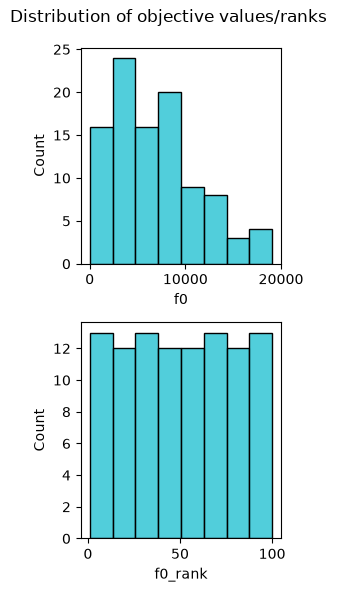
Each xLA feature in pyXla produces as output both visual and numerical outputs. For most features these outputs are returned as a pair.

The numerical output is the first item in the pair:

feat

{'f0_min': 6.320243182647644,
 'f0_max': 19066.8850782852,
 'f0_mean': 6839.651998633828,
 'f0_med': 6204.2294404687345,
 'f0_q1': 3498.9646869908393,
 'f0_q3': 9473.985346242045,
 'f0_sd': 4520.323400836366,
 'f0_skew': 0.6481937541499783,
 'f0_kurt': -0.1579802993935533,
 'f0_rank_min': 1,
 'f0_rank_max': 100,
 'f0_rank_mean': 50.5,
 'f0_rank_med': 50.5,
 'f0_rank_q1': 25.25,
 'f0_rank_q3': 75.75,
 'f0_rank_sd': 29.011491975882016,
 'f0_rank_skew': 0.0,
 'f0_rank_kurt': -1.2002400240024003}

The visual output is the second item in the pair:

plot

For a complete reference of all the xLA features implemented in pyXla see the API reference.