Comparing Knapsack Instances

Download this as a Jupyter notebook

This examples notebook shows how xLA of a discrete optimisation problem: the knapsack problem. It utilises samples provided by the maintainers of pyXla. You can access all the samples here.

For convenience of accessing the samples, we use pyxla.util.load_sample() to load the knapsack instances:

from pyxla.util import load_sample

Change the working directory to src\

%pwd

'/home/docs/checkouts/readthedocs.org/user_builds/pyxla/checkouts/latest/docs/source/guides/examples'

%cd ../../../../src

/home/docs/checkouts/readthedocs.org/user_builds/pyxla/checkouts/latest/src

kp_n10_f20_id42_F1_V1 = load_sample('kp_n10_f20_id42_F1_V1', test=False)
kp_n10_f80_id42_F1_V1 = load_sample('kp_n10_f80_id42_F1_V1', test=False)

The sample kp_n10_f20_id42_F1_V1 has solutions of 10 dimensions hence n10 in its name, a feasibility rate of 20% (from f20), has 1 objective (from F1) and one constraint (from V1).

The second instance kp_n10_f80_id42_F1_V1 differs from the the first with regard to feasibility rate. It has a feasibility rate of 80%.

Violation distribution

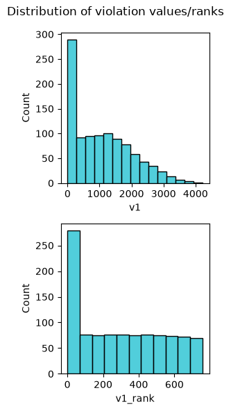
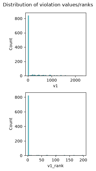
Confirm the feasibility rate using violation distribution (pyxla.util.distr_v()):

from pyxla import distr_v

feat, plot = distr_v(kp_n10_f20_id42_F1_V1)
feat

{'v1_min': 0.0,
 'v1_max': 4215.8,
 'v1_mean': 1062.95234375,
 'v1_med': 945.3,
 'v1_q1': 186.05,
 'v1_q3': 1704.55,
 'v1_sd': 919.413741462782,
 'v1_skew': 0.6162510693993406,
 'v1_kurt': -0.4064585933657159,
 'v1_feas_rate': 0.2001953125,
 'overall_feas_rate': 0.2001953125}

feat, plot = distr_v(kp_n10_f80_id42_F1_V1)
feat

{'v1_min': 0.0,
 'v1_max': 2325.2,
 'v1_mean': 117.65234375,
 'v1_med': 0.0,
 'v1_q1': 0.0,
 'v1_q3': 0.0,
 'v1_sd': 316.0870634890906,
 'v1_skew': 3.2781647150241064,
 'v1_kurt': 11.545774569080045,
 'v1_feas_rate': 0.7998046875,
 'overall_feas_rate': 0.7998046875}

Correlation

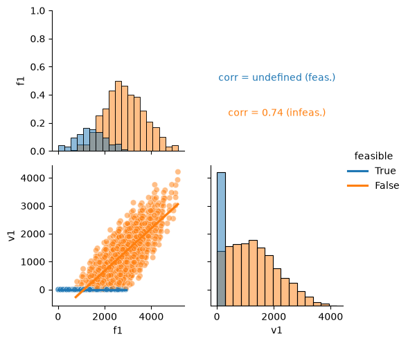
What can pyxla.corr() tell us?

from pyxla import corr

corr_coef, plot = corr(kp_n10_f20_id42_F1_V1)
corr_coef

/home/docs/checkouts/readthedocs.org/user_builds/pyxla/checkouts/latest/src/pyxla/__init__.py:380: ConstantInputWarning: An input array is constant; the correlation coefficient is not defined.
  cor, _ = spearmanr(x, y)

{'v1_f1 (feas.)': 'undefined', 'v1_f1 (infeas.)': '0.74'}

corr_coef, plot = corr(kp_n10_f80_id42_F1_V1)
corr_coef

/home/docs/checkouts/readthedocs.org/user_builds/pyxla/checkouts/latest/src/pyxla/__init__.py:380: ConstantInputWarning: An input array is constant; the correlation coefficient is not defined.
  cor, _ = spearmanr(x, y)

{'v1_f1 (feas.)': 'undefined', 'v1_f1 (infeas.)': '0.55'}

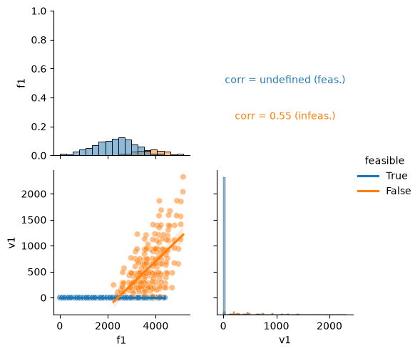
A high correlation between the constraint and the objective leads to a low feasibility rate (20%) as expected since higher profit items tends to have higher weights leading to fewer feasible solutions. Conversely a low correlation between profit and weight leads to a higher feasibility rate (80%).