Neighbouring Change in Feasibility (N∆Feas)

import math

from pyxla import ncf
from pyxla.util import load_data
from pyxla.sampling import HilbertCurveSampler

sphere_sample_all_v = {
    "name": "Sphere",
    "X": HilbertCurveSampler(sample_size=100, dim=1, l_bound=-5, u_bound=5, seed=42),
    "F": lambda x: x**2,
    "V": [lambda x: x**2 - 2, lambda x: 8 * math.sin(20 * x)]
}

sphere_sample_v0 = {
    "name": "Sphere",
    "X": HilbertCurveSampler(sample_size=100, dim=1, l_bound=-5, u_bound=5, seed=42),
    "F": lambda x: x**2,
    "V": [lambda x: x**2 - 2]
}

sphere_sample_v1 = {
    "name": "Sphere",
    "X": HilbertCurveSampler(sample_size=100, dim=1, l_bound=-5, u_bound=5, seed=42),
    "F": lambda x: x**2,
    "V": [lambda x: 8 * math.sin(20 * x)]
}

load_data(sphere_sample_all_v)
load_data(sphere_sample_v0)
load_data(sphere_sample_v1)

WARNING:root:The Hilbert curve with dimension 1 is just a number line. You are sampling around points on a number line.
WARNING:root:The Hilbert curve with dimension 1 is just a number line. You are sampling around points on a number line.
WARNING:root:The Hilbert curve with dimension 1 is just a number line. You are sampling around points on a number line.

The constrained sphere problem has 2 constraints:

(1)\[v_0(x) = x^2 - 2 \leq 0,~\text{and}\]

(2)\[v_1(x) = 8 \cdot \sin(20 \cdot x) \leq 0.\]

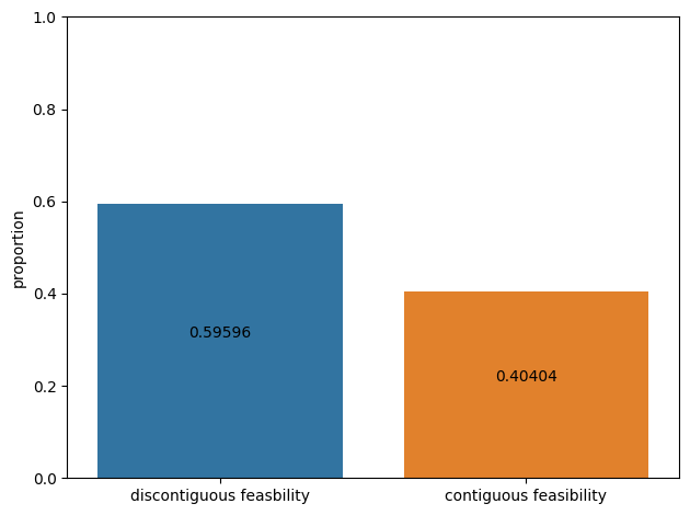
NCF with both constraints:

proportions, plot = ncf(sphere_sample_all_v, title=False)
plot.figure.savefig('ncf-all-v.png', dpi=300)

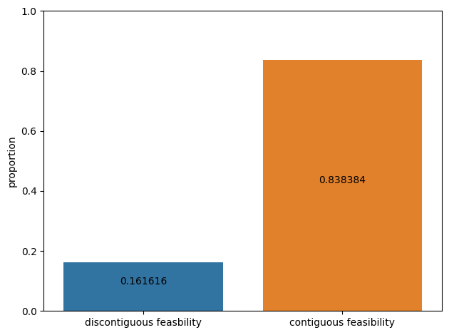
For the spherical constraint:

proportions, plot = ncf(sphere_sample_v0, title=False)
plot.figure.savefig('ncf-v0.png', dpi=300)

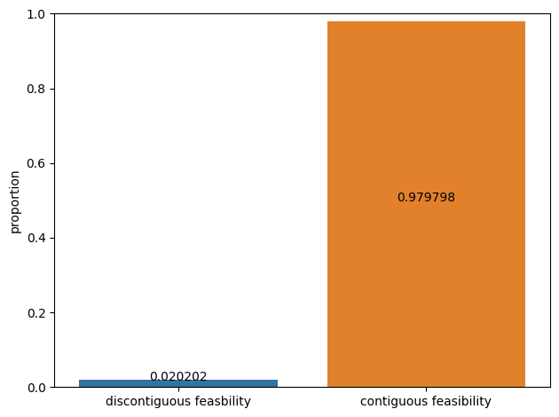
For the sinusodial constraint:

proportions, plot = ncf(sphere_sample_v1, title=False)
plot.figure.savefig('ncf-v1.png', dpi=300)