Analysing an SGD NN Optimisation Trajectory

Simulate the XOR gate using a neural network (NN). Collect the trajectory of SGD when training the NN and analyse it.

Setup NN

seed = 100

import torch
import torch.nn as nn
import numpy as np
import seaborn as sns
import pandas as pd
import torch.nn.init as init

class XOR(nn.Module):
    def __init__(self):
        super(XOR, self).__init__()

        self.layers = nn.Sequential(
            nn.Linear(2, 2),
            nn.Tanh(),
            nn.Linear(2, 1),
        )
    def forward(self, x):
        return self.layers(x)

def weight_init(m):
    '''
    Usage:
        model = Model()
        model.apply(weight_init)
    '''
    
    if isinstance(m, nn.Linear):
        init.xavier_normal_(m.weight.data)
        init.uniform_(m.bias.data)

def get_weights_biases(model: XOR):
    return [
        model.layers[0].weight[0][0].item(),
        model.layers[0].weight[0][1].item(),
        model.layers[0].weight[1][0].item(),
        model.layers[0].weight[1][1].item(),
        model.layers[0].bias[0].item(),
        model.layers[0].bias[1].item(),
        model.layers[2].weight[0][0].item(),
        model.layers[2].weight[0][1].item(),
        model.layers[2].bias[0].item(),
    ]

device = torch.device("cpu")

x_train = torch.tensor([[0,0], [0,1], [1,1], [1,0]], device=device).float()
y_train = torch.tensor([[0], [1], [0], [1]], device=device).float()


x_val = torch.clone(x_train)
y_val = torch.clone(y_train)

torch.manual_seed(seed)
np.random.seed(seed)

model = XOR()
model.apply(weight_init)
model = model.to(device)

lr = 0.1
n_epochs = 1000

optimizer = torch.optim.SGD(model.parameters(), lr=lr)
loss_fn = nn.BCEWithLogitsLoss()

weights = []
losses = []
for epoch in range(n_epochs):
    model.train()

    logits = model(x_train)

    loss = loss_fn(logits, y_train)

    losses.append(loss.item())
    
    loss.backward()

    optimizer.step()

    weights.append(get_weights_biases(model))
    
    optimizer.zero_grad()
    if (epoch % 50 == 0):
        print("Epoch: {0}, Loss: {1}, ".format(epoch, loss.to("cpu").detach().numpy()))

Epoch: 0, Loss: 0.6997735500335693, 
Epoch: 50, Loss: 0.6368666887283325, 
Epoch: 100, Loss: 0.6079322099685669, 
Epoch: 150, Loss: 0.585761308670044, 
Epoch: 200, Loss: 0.566925585269928, 
Epoch: 250, Loss: 0.5497063994407654, 
Epoch: 300, Loss: 0.5328973531723022, 
Epoch: 350, Loss: 0.5154256820678711, 
Epoch: 400, Loss: 0.4956590533256531, 
Epoch: 450, Loss: 0.4689560532569885, 
Epoch: 500, Loss: 0.4196017384529114, 
Epoch: 550, Loss: 0.3432215452194214, 
Epoch: 600, Loss: 0.2689013183116913, 
Epoch: 650, Loss: 0.21145915985107422, 
Epoch: 700, Loss: 0.17034313082695007, 
Epoch: 750, Loss: 0.14094915986061096, 
Epoch: 800, Loss: 0.11939752101898193, 
Epoch: 850, Loss: 0.10311853140592575, 
Epoch: 900, Loss: 0.090479776263237, 
Epoch: 950, Loss: 0.08043112605810165, 

X = pd.DataFrame(weights)
X.columns = ['w0', 'w1', 'w2', 'w3', 'b0', 'b1', 'w4', 'w5', 'b2']
F = pd.DataFrame()
F['train_loss'] = losses
F['epoch'] = list(F.index)

sample = {
    'name': 'xor-sgd',
    'X': X,
    'F': F.drop(columns='epoch'),
    'N': 'X-index' # use index in X to infer neighbourhood
}

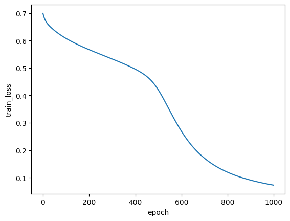
ax = sns.lineplot(F, x='epoch', y='train_loss')

Setup pyXla sample

from pyxla import load_data
import pyxla

load_data(sample)

feat, plot = pyxla.distr_f(sample, title=False)

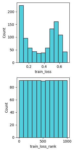
plot.savefig('distr-f-xor-nn-trained.png', dpi=300)

corr, imp, plot = pyxla.X_imp(sample, estimator='ridge', alpha=1, n_repeats=30, seed=seed, suptitle=False)

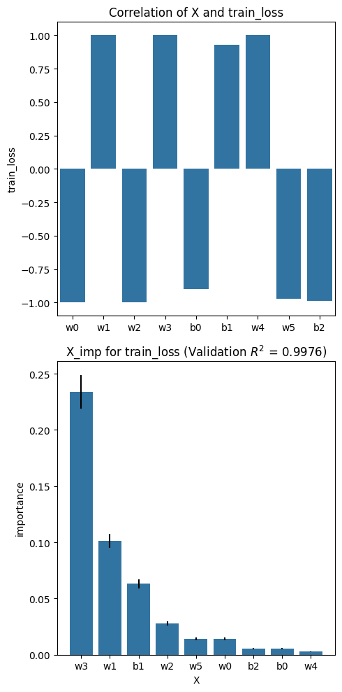
plot.savefig('x-imp-xor-nn-trained.png', dpi=300)

corr, plot = pyxla.fdc(sample)

WARNING:root:No D file is present, thus, computing the D file... Computing an entire D file can be time consuming. Instead, you can call the function with the keyword argument `compute_D_file` set to `False` to speed up computation, as only the required distances will be calculated.
INFO:root:D file has been loaded to the current sample and is saved to ./xor-sgd_D.csv

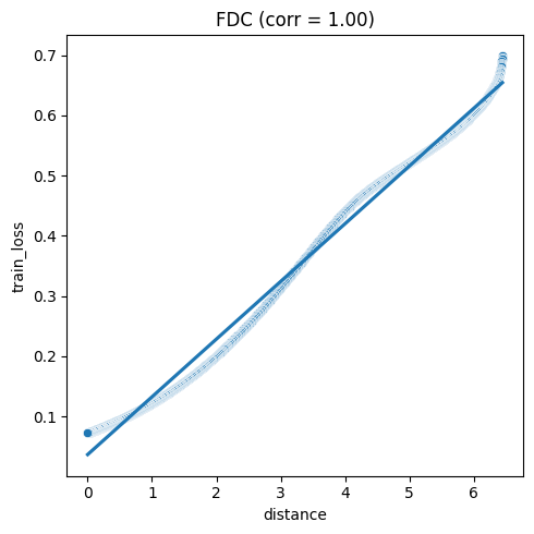
plot.savefig('fdc-xor-nn-trained.png', dpi=300)

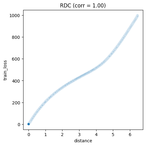
corr, plot = pyxla.rdc(sample)

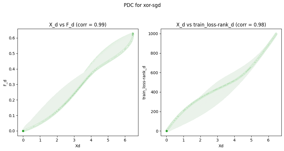
corr, plot = pyxla.pdc(sample)

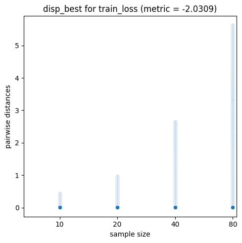
pyxla.disp_best(sample)

/home/toni/Projects/pyxla-wg/src/pyxla/__init__.py:1409: RuntimeWarning: divide by zero encountered in log
  forward = lambda x: np.log(x / init_percentage) / np.log(growth_factor)

({'train_loss': np.float64(-2.030872834502893)},
 <Figure size 500x500 with 1 Axes>)

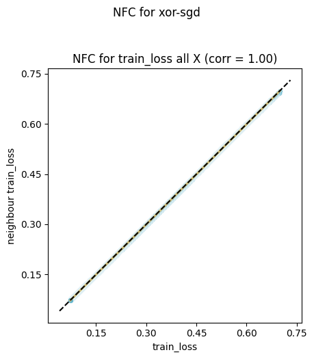
corr, plot = pyxla.nfc(sample)

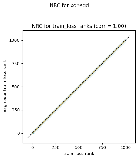
corr, plot = pyxla.nrc(sample)