Correlation of Values (corr)

Sphere Problem

import math

from pyxla import load_data, corr
from pyxla.util import load_sample
from pyxla.sampling import HilbertCurveSampler

sphere_sample = {
    "name": "Sphere",
    "X": HilbertCurveSampler(sample_size=100, dim=1, l_bound=-5, u_bound=5, seed=42),
    "F": lambda x: x**2,
    "V": [lambda x: x**2 - 2, lambda x: 8 * math.sin(20 * x)]
}

load_data(sphere_sample)

WARNING:root:The Hilbert curve with dimension 1 is just a number line. You are sampling around points on a number line.

corrs, plot = corr(sphere_sample)

/home/toni/Projects/pyxla-wg/src/pyxla/__init__.py:376: ConstantInputWarning: An input array is constant; the correlation coefficient is not defined.
  cor, _ = spearmanr(x, y)

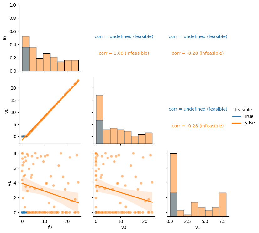
corrs

{'v0_f0 (feasible)': 'undefined',
 'v0_f0 (infeasible)': '1.00',
 'v1_f0 (feasible)': 'undefined',
 'v1_f0 (infeasible)': '-0.28',
 'v1_v0 (feasible)': 'undefined',
 'v1_v0 (infeasible)': '-0.28'}

NK Problem

The corr feature is very useful for multiobjective problems.

An NK instance with 3 objectives and 2 constraints is exemplified below:

# change directory to access samples
%cd ../../..
nk = load_sample('nk_n14_k2_id5_F3_V2')

/home/toni/Projects/pyxla-wg/docs

nk['V'] = None
nk['numV'] = 0

corr, plot = corr(nk)

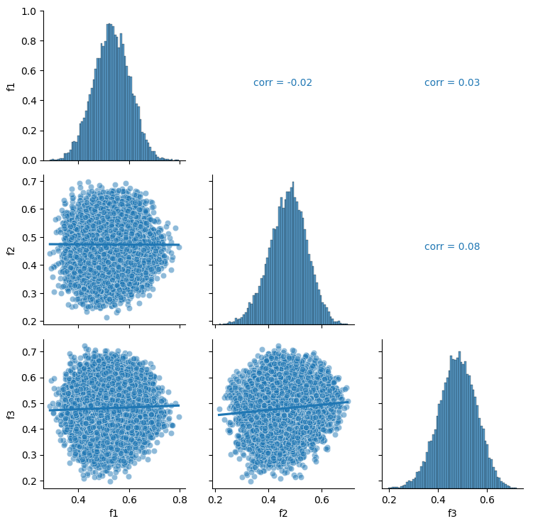
plot.savefig('corr-nk-f3', dpi=300)

corr

{'f2_f1 (feasible)': '-0.38',
 'f2_f1 (infeasible)': '-0.01',
 'f3_f1 (feasible)': '-0.28',
 'f3_f1 (infeasible)': '0.03',
 'v1_f1 (feasible)': 'undefined',
 'v1_f1 (infeasible)': '-0.02',
 'v2_f1 (feasible)': 'undefined',
 'v2_f1 (infeasible)': '0.02',
 'f3_f2 (feasible)': '0.39',
 'f3_f2 (infeasible)': '0.08',
 'v1_f2 (feasible)': 'undefined',
 'v1_f2 (infeasible)': '-0.09',
 'v2_f2 (feasible)': 'undefined',
 'v2_f2 (infeasible)': '0.01',
 'v1_f3 (feasible)': 'undefined',
 'v1_f3 (infeasible)': '0.11',
 'v2_f3 (feasible)': 'undefined',
 'v2_f3 (infeasible)': '0.06',
 'v2_v1 (feasible)': 'undefined',
 'v2_v1 (infeasible)': '-0.22'}